Benjamin Ahlbrecht - Early Breast Cancer Detection using Deep Learning Techniques

‹‹ Previous

10638_L

Next ››

Figure 1: Mammogram screening images of individual patients. Highlighted regions indicate areas of potentially cancerous tissue. A combination of true positives, false positives, false negatives, and true negatives are included.

Motivation

Mammograms are routine screenings recommended for woman over the age of 40 in the hopes of detecting breast cancer early. Given the recent advances in deep learning, specifically convolutional neural networks (CNNs), there has been increased interest in creating computer-aided detection and diagnosis (CAD) systems to help detect and segment cancerous tissue in the hopes of both improving patient outcomes and reducing costs and labor associated with reading and interpreting mammograms.

Here, we leverage the EfficientNet-B4 network [1], pretrained on the ImageNet dataset [2] to classify mammogram image screenings as either malignant or benign. For each patient, we aggregate mammogram screenings and predict whether breast cancer exists in either breast.

Dataset

In this work, we use the RSNA Screening Mammography Breast Cancer Detection dataset found on Kaggle. The compressed dataset has a total size of 314.72 GB. Mammography images are provided in DICOM format. A corresponding metadata file is provided in CSV format. There are a total of \(54\, 706\) mammogram images with \(53\, 548\) being cancer negative (benign), meaning that only about 2% of images provided are cancer positive. We describe later how we deal with strongly unbalanced classes utilizing oversampling and data augmentation.

Data Processing

There are a number of steps necessary before images are prepared for ingestion by our model. To ensure adaquate performance, we both window and normalize each image. Additionally, we crop and resize each image to speed up model training and to alleviate computational constraints

Windowing DICOM Images

Patient images are provided in the DICOM standard file format, which stores 16 bit mammogram images encoded in either the JPEG 2000 or the JPEG lossless format. We process these images on the GPU to accelerate model training utilizing the NVIDIA Data Loading Library (DALI).

Since DICOM images contain 12 or 16 unique values (bits) per pixel, they contain far more information than the more standard 8 bit images. A standard 8 bit image may contain \(2^8 = 256\) bits per pixel. On the other hand, a 16 bit image may contain up to \(2^{16} = 65\,536\) bits per pixel, which is 256 times the number of unique values! We can apply windowing techniques emphasize certain structures present in high bitrate mammogram images. Windowing has two parameters:

The window center, \(w_\text{center}\) is the intensity at which we wish to emphasize structures.
The window width, \(w_\text{width}\) specifies the range above and below the center pixel values which we consider

Together, we utilize pixels within the range \(w_\text{center} \pm w_\text{width}\). We clip values above and below the range. To illustrate, consider a flattened image \(\mathcal{X} = \{x_1, x_2, \ldots, x_n\}\). For a given pixel value, \(x_j\), we can apply windowing via the following piecewise function to update the value of \(x_j\):

\[\begin{equation} x_j \leftarrow \begin{cases} w_\text{center} - w_\text{width} &\text{if } x_j < w_\text{center} - w_\text{width} \\ w_\text{center} + w_\text{width} &\text{if } x_j > w_\text{center} + w_\text{width} \\ x_j &\text{Otherwise} \end{cases} \end{equation}\]

Normalizing Pixel Values

It is common practice in machine learning to normalize your input features. This is necessary to standardize the range of values to ensure our model can learn properly. We do this by simply applying min-max normalization to each pixel in an image. Given that \(X_\text{min} = \min\{x_1, x_2, \ldots, x_n\}\) is the minimum value in an image and \(X_\text{max} = \max\{x_1, x_2, \ldots, x_n\}\) is the maximum value in an image, we can re-scale and update a given pixel value \(x_j\) accordingly:

\[\begin{equation} x_j \leftarrow \frac{x_j - X_\text{min}}{X_\text{max} - X_\text{min}} \end{equation}\]

Image Cropping and Resizing

Since mammogram images have a significant amount of background space, we crop each image to exclude the background pixels. This is done by summing across each row and column within an image. If a given sum is 0, we simply remove the respective row or column without any pixel intensity.

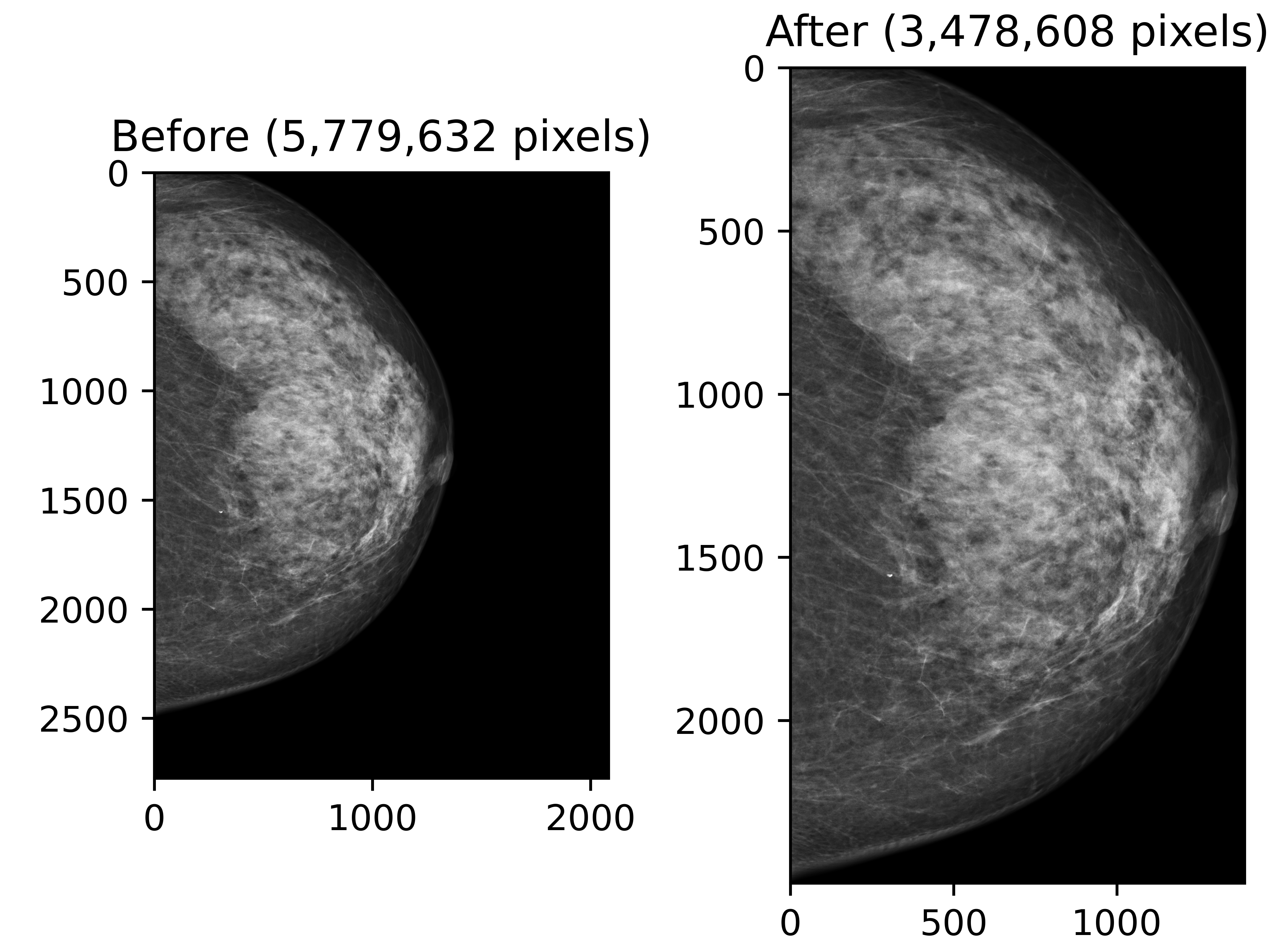
Auto-Cropped Image — **Figure 2:** Removing unnecessary whitespace reduces number of pixels present by 38%.

In addition to cropping each image, we resize the images to a constant width and height. This ensures that we can feed a batch of images into the model and alleviates some computational constraints that would be present otherwise. By examining a subset of the training images, we determine that the average aspect ratio is 1.91. Thus, by setting a constant width of 500 pixels, we obtain a respective height of 955 pixels.

Model Building

As mentioned previously, we build off of the EfficientNet-B4 model pretrained from the ImageNet dataset. Since the ImageNet dataset has 1000 classes, we replace the classification layer with a single neuron, whose output represents the probability of an mammography image containing cancerous tissue. Moreover, we disable training on the initial convolutional blocks in the network following the assumption that the pre-trained network learned more general features of images. Thus, we enable training on the last block to fine tune the learned features for cancer detection.


======================================================================
Layer (type:depth-idx)                        Param #
======================================================================
├─Sequential: 1-1                             --
|    └─Conv2dNormActivation: 2-1              --
|    |    └─Conv2d: 3-1                       (1,296)
|    |    └─BatchNorm2d: 3-2                  (96)
|    |    └─SiLU: 3-3                         --
|    └─Sequential: 2-2                        --
|    |    └─MBConv: 3-4                       (2,940)
|    |    └─MBConv: 3-5                       (1,206)
|    └─Sequential: 2-3                        --
|    |    └─MBConv: 3-6                       (11,878)
|    |    └─MBConv: 3-7                       (18,120)
|    |    └─MBConv: 3-8                       (18,120)
|    |    └─MBConv: 3-9                       (18,120)
|    └─Sequential: 2-4                        --
|    |    └─MBConv: 3-10                      (25,848)
|    |    └─MBConv: 3-11                      (57,246)
|    |    └─MBConv: 3-12                      (57,246)
|    |    └─MBConv: 3-13                      (57,246)
|    └─Sequential: 2-5                        --
|    |    └─MBConv: 3-14                      (70,798)
|    |    └─MBConv: 3-15                      (197,820)
|    |    └─MBConv: 3-16                      (197,820)
|    |    └─MBConv: 3-17                      (197,820)
|    |    └─MBConv: 3-18                      (197,820)
|    |    └─MBConv: 3-19                      (197,820)
|    └─Sequential: 2-6                        --
|    |    └─MBConv: 3-20                      (240,924)
|    |    └─MBConv: 3-21                      (413,160)
|    |    └─MBConv: 3-22                      (413,160)
|    |    └─MBConv: 3-23                      (413,160)
|    |    └─MBConv: 3-24                      (413,160)
|    |    └─MBConv: 3-25                      (413,160)
|    └─Sequential: 2-7                        --
|    |    └─MBConv: 3-26                      (520,904)
|    |    └─MBConv: 3-27                      (1,159,332)
|    |    └─MBConv: 3-28                      (1,159,332)
|    |    └─MBConv: 3-29                      (1,159,332)
|    |    └─MBConv: 3-30                      (1,159,332)
|    |    └─MBConv: 3-31                      (1,159,332)
|    |    └─MBConv: 3-32                      (1,159,332)
|    |    └─MBConv: 3-33                      (1,159,332)
|    └─Sequential: 2-8                        --
|    |    └─MBConv: 3-34                      1,420,804
|    |    └─MBConv: 3-35                      3,049,200
|    └─Conv2dNormActivation: 2-9              --
|    |    └─Conv2d: 3-36                      802,816
|    |    └─BatchNorm2d: 3-37                 3,584
|    |    └─SiLU: 3-38                        --
├─AdaptiveAvgPool2d: 1-2                      --
├─Sequential: 1-3                             --
|    └─Dropout: 2-10                          --
|    └─Linear: 2-11                           1,793
|    └─Sigmoid: 2-12                          --
======================================================================
Total params: 17,550,409
Trainable params: 5,278,197
Non-trainable params: 12,272,212
======================================================================

Figure 3: Adapted EfficientNet-B4 model. Only blocks following Sequential: 2-8 have their gradients enabled for learning.

Data Loading and Augmentation

To prepare for model training and validation, we create a data loader to automatically process, retrieve, and optionally augment batches of patient images. We utilize a batch size of 8, meaning that we grab all images corresponding to 8 randomly selected prediction IDs. Prediction IDs Each prediction ID is associated with, on average, 2-3 images, meaning that a batch size of 8 will tend to draw 16-24 images that will be fed at once. Batches are drawn in such a manner since the model will be evaluated on both individual predictions and predictions aggregated over the prediction ID.

Patient Vs. Prediction Id — **Figure 4:** A single patient ID is split into two prediction IDs corresponding to left and right breast laterality. Each prediction ID is assigned the same label corresponding to the ground truth of whether the breast contains cancerous tissue. Additionally, each prediction ID may have 2-3 images, on average, from various mammogram views.

Due to heavily unbalanced classes, we employ a weighted random sampler to equally sample benign and malignant prediction IDs within the training and validation sets. This ensures we do not overtrain on benign examples, forcing the model to learn malignant features.

Images in the training dataset are augmented randomly to diversify the training set, aiding the model to better generalize given the small sample size of malignant cancer observations. We perform a number of random augmentations, including random vertical and horizontal image flips, random image rotations, translations, and shearing.

Data Pipeline — **Figure 5:** The full data processing and ingestion pipeline. We created weighted random samplers given the labels found in the training and validation metadata such that there is an equal chance of sampling benign and malignant prediction IDs. To train the model, we request a series of training batches. With each training batch, we preprocess and augment the image. The same steps are performed for the validation dataset excluding data augmentation.

Model Training and Validation

We train the model over a maximum of 50, utilizing a batch size of 8 prediction IDs. The ADAM optimizer is initialized with a learning rate of \(\alpha = 1 \times 10^{-3}\). If the validation loss does not improve after a single epoch, the learning rate is reduced by a factor of \(0.10\) with a minimum learning rate of \(\alpha_\text{min} = 1 \times 10^{-6}\). Additionally, if the validation loss does not improve by a minimum of \(0.01\) after 8 epochs, then we stop training and retrieve the model with the lowest validation loss.

Training History — **Figure 6:** The training and validation loss curves for the proposed model. The weights from epoch 10 are retrieved due to the early stopping condition.

After the model is fine-tuned to predict whether an individual image is malignant or benign, we define a simple algorithm to aggregate multiple individual predictions in a single aggregated prediction. To do this, we take a weighted average of each probability and determine the probability at-least one image is positive. Specifically, if we have a set of individual probabilities, \(\mathcal{P} = \{p_1, p_2, \ldots, p_n\}\), we define the weighted average as \(\bar{P} = \frac{1}{n} \sum_{p \in \mathcal{P}}p^2\). Then, we determine the aggregated probability, \(P_\text{agg}\):

\[\begin{equation} P_\text{agg} = 1 - (1 - \bar{P})^n \end{equation}\]

Evaluation Metrics

Since the classes (cancer positive Versus cancer negative) are inherently unbalanced, accuracy becomes an uninformative evaluation metric. Instead, we utilize the recall, precision, and the \(F_1\)-score for model evaluation.

Precision quantifies the proportion of cancer positive classifications that we correctly classified as cancer positive. If TP, TN, FP, FN are the number of true positives, true negatives, false positives, and false negatives, respectively, then we can define the precision as follows:

\[\begin{equation} \text{Precision} = \frac{\text{TP}}{\text{TP} + \text{FP}} \end{equation}\]

Recall, on the other hand, quantifies the proportion of cancer positive classifications out of the total number of cancer positive classifications:

\[\begin{equation} \text{Recall} = \frac{\text{TP}}{\text{TP} + \text{FN}} \end{equation}\]

In a classification scenario, we often wish to strike a balance between the recall and precision. In this case, we can take the harmonic mean between precision and recall to compute the \(F_1\)-score:

\[\begin{equation} \text{F}_1 = 2 \frac{\text{Precision} \cdot \text{Recall}}{\text{Precision} + \text{Recall}} \end{equation}\]

Metric	Instance Classifier	Aggregator Classifier
Precision	0.623	0.638
Recall	0.889	0.846
\(F_1\)-Score	0.735	0.727

Figure 7: The evaluation metrics of the instance and aggregator classifiers.

Since our recall is higher than our precision, we can tell that the model is far better at identifying false negatives than false positives. This can be verified in the decision matrices:

Instance Confusion Matrix — **Figure 8:** Confusion matrices for the instance-based model and the aggregator.

Aggregator Confusion Matrix — **Figure 8:** Confusion matrices for the instance-based model and the aggregator.

Class Activation Mapping

Class activation mapping (CAM) is a semi-supervised learning method for providing explainability to convolutional neural networks. It works by determining the local influence of each relative pixel location in the input image [3]. We begin by discussing the theory behind CAMs, discussing its computation and its relationship to traditional classification in a CNN. Next, we'll examine a few examples of CAMs produced by the model.

Theory and Computation

In order to produce a CAM, it is assumed that our CNN ends with a global average pooling layer prior to a dense sequential block for classification. Suppose we feed an input image \(I \in \mathbb{R}^{h \times w}\) with height and width, \(h\) and \(w\).

Feeding images into the CNN extracts features, creating features maps. We denote the set of last feature maps immediately prior to the global average pooling (GAP) as \(\mathcal{f} = \{f_1, \ldots, f_k \}\), where \(f_i\) is matrix such that \(f_i \in \mathbb{R}^{n \times m}\). GAP averages each feature map to produce a single vector of values: \(F = \{F_1, \ldots, F_k\}\), where \(F_i = \frac{1}{n \times m}\sum_{x \in \mathcal{X}} \sum_{y \in \mathcal{Y}} f_i(x, y)\).

To make a binary prediction (benign or malignant), we add a single classification neuron proceeding the GAP layer with learned weights \(w = \{w_1, \ldots, w_k\}\). We define the input to the classification neuron, \(S_\text{cancer}\) as the weighted sum between the GAP values and the corresponding weights: \(S_\text{cancer} = \sum_{k \in \mathcal{K}} F_k w_k\). In order to determine the output of the neuron, a sigmoid activation is simply applied. Specifically, the estimate of the input image being cancerous is \(P_\text{Cancer} = \sigma(S_\text{cancer})\).

CNN Classification — **Figure 9:** Classification for an input image \(I\) with 3 example feature maps. Global average pooling averages each feature map into \(\{F_1, F_2, F_3\}\). A transfer function combines each average with a learned weight to produce the input to the classification neuron, \(S_\text{cancer}\). A sigmoid activation function converts the input into a probability, \(P_\text{cancer}\).

Instead of taking the conventional classification route, CAM seeks to compute the local activation importance for each relative position in the input image. Suppose that the value of a given pixel location in the last set of feature maps is denoted by \(f_i(x, y)\). For a given pixel location, \((x, y)\), we apply a weighted sum across the weights learned by the GAP layer: \(M(x, y) = \sum_{k \in \mathcal{K}} f_k(x, y) w_k\). We refer to this as the local image importance, quantifying the activation for pixel location \((x, y)\) in the last set of feature maps. Performing this procedure across all pixels in the feature maps generate the class activation matrix.

To better isolate potentially cancerous regions, we threshold the CAM image by only retaining local activation values above the mean and one standard deviation. All other values are set to 0. In order to convert the class activation matrix to the class activation map, the class activation matrix is simply upscaled to the original image size and interpolated to ensure that it is smooth. To display the CAM, it may be overlayed the original image or presented alongside it.

CAM Classification — **Figure 10** CAM generation and classification for an input image \(I \in \mathbb{R}^{h \times w}\). The local classification importance for each pixel in the feature map is determined by performing a weighted sum for the same pixel location in each feature map. Performing this across each pixel generates the class activation matrix. The matrix may be averaged to retrieve the input to the classification neuron or upscaled and interpolated to retrieve the CAM.

To illustrate that the CAM method is essentially an alternative route to classification, we can compute the classification result directly from the class activation matrix. This is done by averaging the class activation matrix, producing \(S_\text{cancer}\), the input of the classification neuron. As shown before, we convert this input into a probability by applying a sigmoid activation function, \(P_\text{cancer} = \sigma(S_\text{cancer})\).

Conclusion & Future Work

We perform breast cancer detection using the pretrained EfficientNet-B4 model. The DICOM are preprocessed on the GPU using NVIDIA DALI. Training observations are augmented to increase model generalization. We implement CAM to provide model explainability and to suggest regions of interest even in the case of a false negative. Overall, the model achieves an \(F_1\)-score of 0.735. Additionally, we aggregate the individual observations for each prediction ID, achieving a similar \(F_1\)-score of 0.727.

There are a number of potential areas to explore to improve model performance which we explore below:

In addition to model explainability, we can utilize the CAM to implement semantic segmentation, where-in we associate every pixel in a given input image with a classification. Some proposed methodologies are C-CAM [4] and MixupCAM [5]
A better aggregation algorithm can be implemented or learned. Currently, we just average the uncentered 2nd moment of a vector of probabilities, fit a binomial distribution according to that probability, and compute the probability of at-least one success (malignant). We can view this as a multiple instance learning problem. As such, we may be able to adjust the network to make a single prediction for an arbitrary number of input images.
Fine-tuning hyperparameters may strongly increase model performance. We could start by implementing an learning rate tuner to estimate the optimal initial learning rate. Next, we can experiment with the number of layers we freeze or unfreeze. Currently, we train only about 30% of the network. Unfreezing previous layers may help the network learn general features necessary for identifying malignant tissue. Gradient accumulation will help us back-propogate through a sub-batches of images, alleviating our current VRAM restriction.
Lastly, it may help to experiment with different data augmentation policies. For instance, the model we have has trouble predicting tumors from heterogeneously dense and extremely dense breast tissue. Altering the contrast, for example, may help the model generalize to denser breast tissue.

Early Breast Cancer Detection using Deep Learning Techniques

References

- Tan, Mingxing, and Quoc Le. "Efficientnet: Rethinking model scaling for convolutional neural networks." International conference on machine learning. PMLR, 2019.
- Deng, Jia, et al. "Imagenet: A large-scale hierarchical image database." 2009 IEEE conference on computer vision and pattern recognition. Ieee, 2009.
- Zhou, Bolei, et al. "Learning deep features for discriminative localization." Proceedings of the IEEE conference on computer vision and pattern recognition. 2016.
- Chen, Zhang, et al. "C-CAM: Causal CAM for Weakly Supervised Semantic Segmentation on Medical Image." Proceedings of the IEEE/CVF Conference on Computer Vision and Pattern Recognition. 2022.
- Chang, Yu-Ting, et al. "Mixup-cam: Weakly-supervised semantic segmentation via uncertainty regularization." arXiv preprint arXiv:2008.01201 (2020).
Additional Resources
- Singh, Anuj Kumar, and Bhupendra Gupta. "A novel approach for breast cancer detection and segmentation in a mammogram." Procedia Computer Science 54 (2015): 676-682.
- Sechopoulos, Ioannis, Jonas Teuwen, and Ritse Mann. "Artificial intelligence for breast cancer detection in mammography and digital breast tomosynthesis: State of the art." Seminars in Cancer Biology. Vol. 72. Academic Press, 2021.
- Marques, Gonçalo, Deevyankar Agarwal, and Isabel de la Torre Díez. "Automated medical diagnosis of COVID-19 through EfficientNet convolutional neural network." Applied soft computing 96 (2020): 106691.
- Nayak, Dillip Ranjan, et al. "Brain tumor classification using dense efficient-net." Axioms 11.1 (2022): 34.
- Abdelrahman, Leila, et al. "Convolutional neural networks for breast cancer detection in mammography: A survey." Computers in biology and medicine 131 (2021): 104248.
- Shen, Li, et al. "Deep learning to improve breast cancer detection on screening mammography." Scientific reports 9.1 (2019): 12495.
- Zebari, Dilovan Asaad, et al. "Systematic review of computing approaches for breast cancer detection based computer aided diagnosis using mammogram images." Applied Artificial Intelligence 35.15 (2021): 2157-2203.
- Elgendi, Mohamed, et al. "The effectiveness of image augmentation in deep learning networks for detecting COVID-19: A geometric transformation perspective." Frontiers in Medicine 8 (2021): 629134.
- Jung, Hyungsik, and Youngrock Oh. "Towards better explanations of class activation mapping." Proceedings of the IEEE/CVF International Conference on Computer Vision. 2021.
- Implementation of Class Activation Map (CAM) with PyTorch
- Downloading and Preprocessing Medical Images in Bulk: DICOM to NumPy with Python
- A Matter of Grayscale: Understanding Dicom Windows